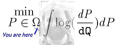
New thought:
Estimate the Infected at time t, not just with the new infections observed at time t but add the infections that are observed the following few ( less than 7 or 8 days) days. Let this lead be another parameter. — Idea!
Data from Chile:
library(tidyverse)
library(zoo)
raw_tibble <- read_csv("https://raw.githubusercontent.com/MinCiencia/Datos-COVID19/master/output/producto5/TotalesNacionales_T.csv")
extract just what’s needed with the function get_sir
sum_ahead <- function(v,lead=1) {
    if (lead > 0) {
        df <- tibble(V1=v)
        df$V2 <- rollsum(lead(df$V1), lead, align="left", fill = NA) + df$V1
        V3 <- df[['V2']]
        df1 <- df %>% filter(is.na(V2)) %>% mutate(V2=rev(cumsum(rev(V1))))
        V3[is.na(V3)] <- df1$V2
    }
    else V3 <- v
    V3
}

get_sir <- function(tib,newI,newD,lead=0) {
   nI <- tib[[newI]]
   nD <- tib[[newD]]
   R <- cumsum(nI+nD)
   n_days <- length(R)
   I <- sum_ahead(nI,lead)
   N_tot <- R[n_days] + I[n_days]
   S <- N_tot - I - R
   R0 <- 1 + diff(c(0,I))/diff(c(1,R))
   sir <- tibble(t=as.Date(tib[[1]],format="%Y-%m-%d"),
                 S=S, I=I, R=R, R0=R0)
   sir
}
Let’s try it,
rt <- tibble(t=raw_tibble[[1]], newI=raw_tibble[[8]],
             newD=diff(c(0,raw_tibble[[5]])))
pR0 <- function(lead=0,df=15,tib=rt) {
  sir <- get_sir(tib,'newI','newD',lead)
  R0 <- sir$R0
  R0[R0==Inf | is.nan(R0)] <- 1   # regularize the Inf
  n_days <- length(R0)
  plot(R0,type="l",xlab="days after 2020-03-03",
        main=paste("Chile: R0, lead=",lead," smoothed with df=",df))
  abline(h=1,col="red")
  lines(smooth.spline(x=1:n_days,y=R0,df=15),col="blue")
}
first with no lead
pR0()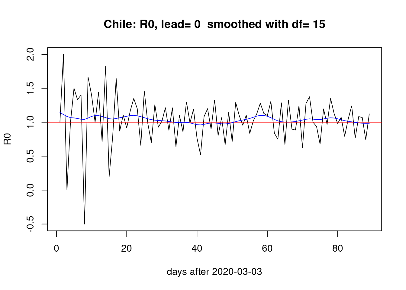 With a week of lead,
pR0(lead=7)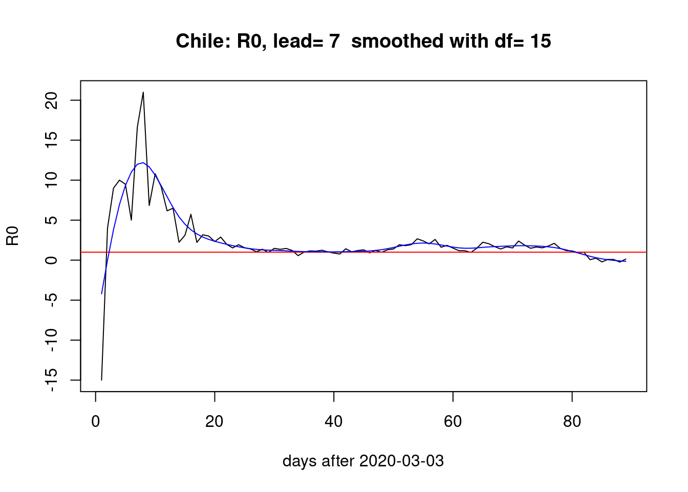 With a lead of four days,
pR0(lead=4)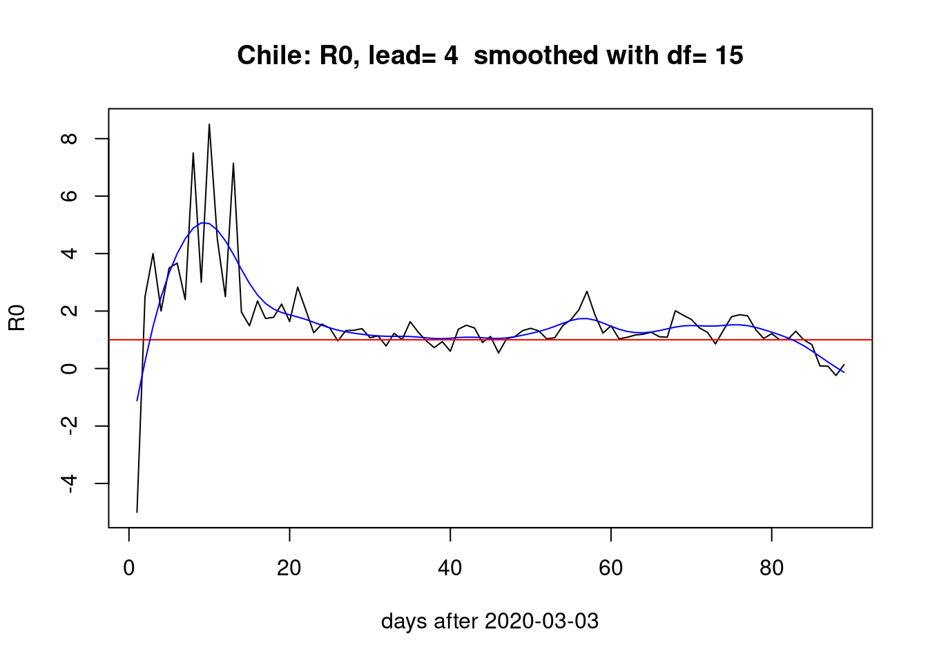
and just two days,
pR0(lead=2)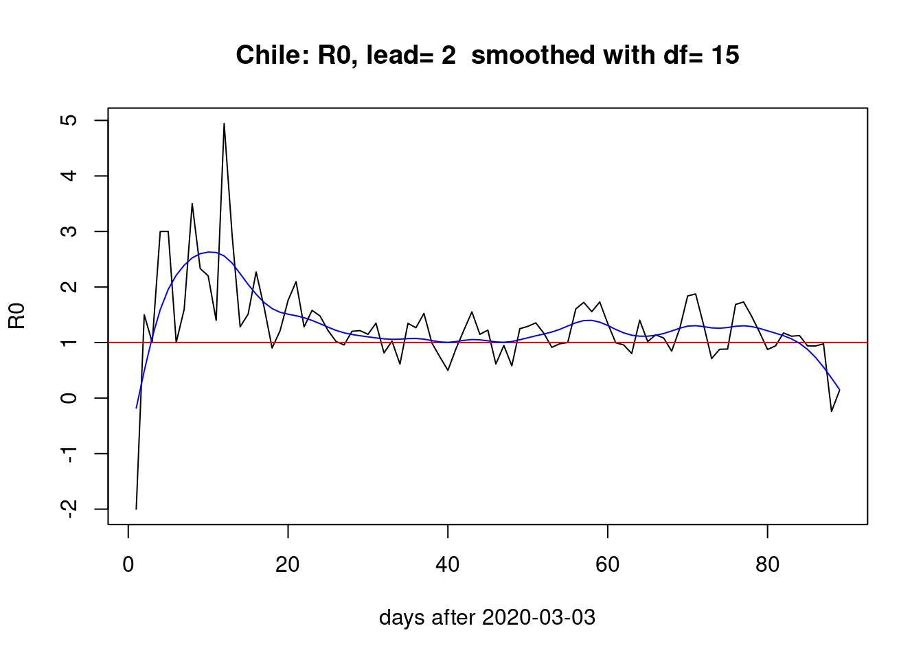
Conclusion
When we estimate the Infectives at time \(t\) by accumulating the new observed cases a lead number of days ahead, we observe that the bump the first month and then two smaller bumps the last month remain stable across changes in the lead parameter.