Get \(R_{0}\)
First we need to provide a .csv file with data.
Data from Chile:
library(tidyverse)
raw_tibble <- read_csv("https://raw.githubusercontent.com/MinCiencia/Datos-COVID19/master/output/producto5/TotalesNacionales_T.csv")
S,I,R estimation
We take the Infectives at time \(t\) to be the new observed cases at time \(t\).
The Removed at time \(t\) will include all of the observed deaths up to time \(t\) plus the total observed infections up to time \(t-\gamma\) where \(\gamma = 0,1,\ldots\) is a parameter modeling the expected number of days between an (primary) infected individual shows symptoms and the time that and indidual infected by the primary (a secondary infection) shows symptoms. For covid19 this is observed to be roughly \(7.5\pm 3.4\) days.
get_sir <- function(tib,newI,newD,gamma=0) {
   nI <- tib[[newI]]
   nD <- tib[[newD]]
   r0 <- cumsum(nI+nD)
   n_days <- length(r0)
   R <- numeric(n_days)
   if (gamma == 0) R[(gamma+1):n_days] <- r0[1:(n_days-gamma)]
   else R[(gamma+1):n_days] <- r0[1:(n_days-gamma)] + nD[(gamma+1):n_days]
   N_tot <- R[n_days] + nI[n_days]
   S <- N_tot - nI - R
   R0 <- 1 + diff(c(0,nI))/diff(c(1,R))
   sir <- tibble(t=as.Date(tib[[1]],format="%Y-%m-%d"),
                 S=S, I=nI, R=R, R0=R0)
   sir
}
Choice of Population Size: \(N\)
The total size of the population is variable over time and difficult to estimate. The SIR model assumes \(N\) constant, and \(N = S+I+R\) for all times (days), thus, the basic reproductive number \(R_{0}\) is independent of \(N\). This may sound counter intuitive but it is clear once you remember that \(R_{0}\) only depends on the increments of \(I\) and \(R\) as we now show.
From the three basic equations of the SIR model, we have
\[ R_{0} = \frac{a}{b} S = \frac{-\delta S}{\delta R}. \]
Hence, from the assumption that \(N\) is constant, \(0=\delta N = \delta S + \delta I + \delta R\) we obtain that,
\[R_{0} = 1 + \frac{\delta I}{\delta R}.\] In the function get_sir above, we just set the total population size so that the last day we end up with no Susceptibles.
rt <- tibble(t=raw_tibble[[1]], newI=raw_tibble[[8]],
newD=diff(c(0,raw_tibble[[5]])))
sir0 <- get_sir(rt,'newI','newD')
R0 <- sir0$R0
n_days <- length(R0)
plot(R0,type="l",main="Chile: R0, lag=0, smoothed with df=15",
xlab="days after March 3. 2020")
abline(h=1,col="red")
lines(smooth.spline(x=1:n_days,y=R0,df=15),col="blue")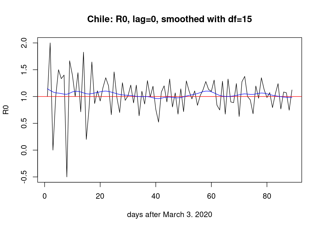 The signal is very weak but recoverable.
We collect the last four lines of r code into a function
to look at the effect of changing the parameter gamma.
The signal is very weak but recoverable.
We collect the last four lines of r code into a function
to look at the effect of changing the parameter gamma.
pR0 <- function(g=0,df=15,tib=rt) {
  sir <- get_sir(tib,'newI','newD',gamma=g)
  R0 <- sir$R0
  R0[1:(g+1)] <- 1   # regularize the Inf
  n_days <- length(R0)
  plot(R0,type="l",xlab="days after 2020-03-03",
        main=paste("Chile: R0, lag=",g," smoothed with df=",df))
  abline(h=1,col="red")
  lines(smooth.spline(x=1:n_days,y=R0,df=15),col="blue")
}
Seven days lag:
pR0(g=7)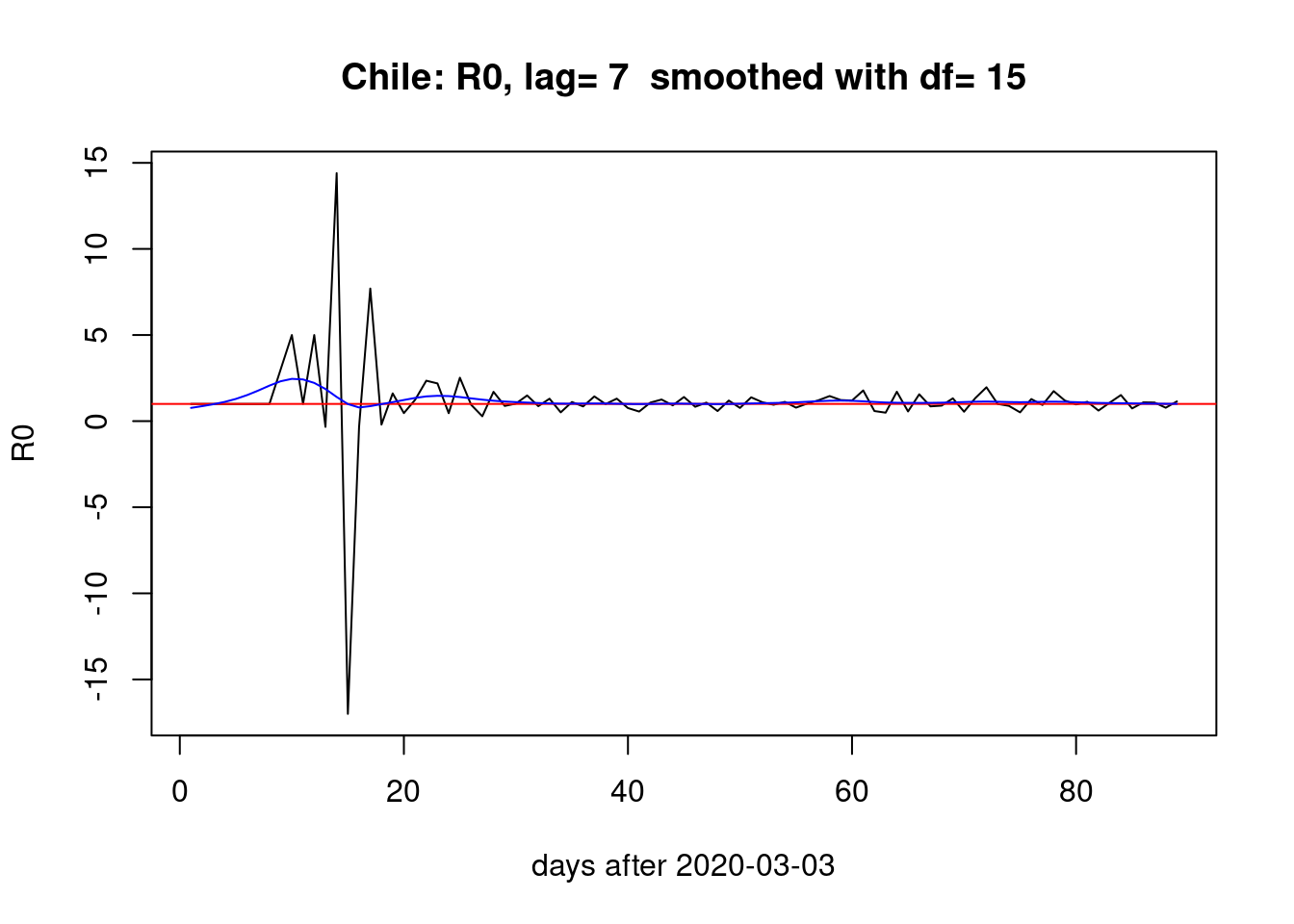
Four days lag:
pR0(g=4)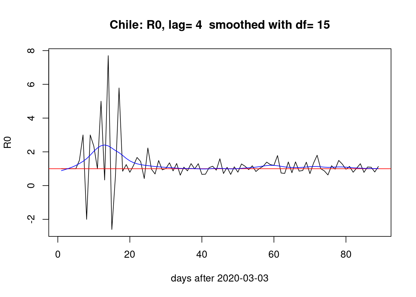
Two days lag:
pR0(2)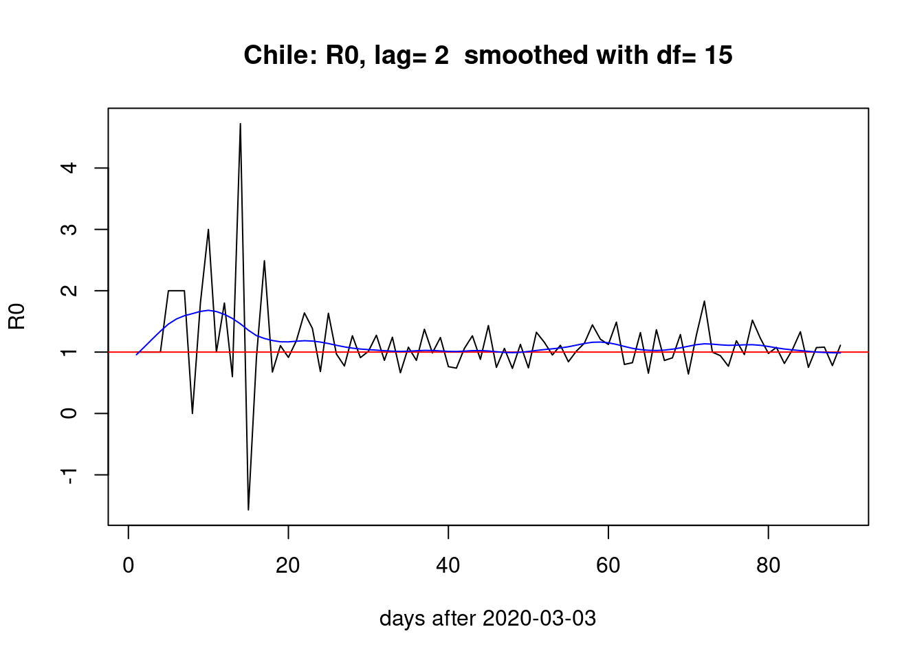
One day lag:
pR0(1)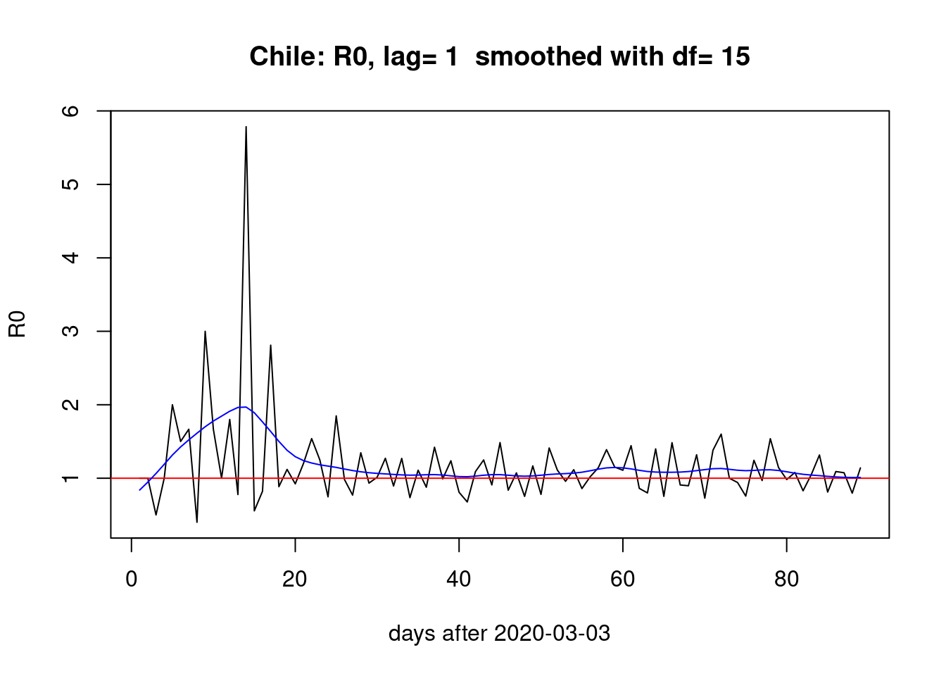
Conclusion
The choice of lag (i.e. the \(\gamma\) parameter) does affect the estimation of \(R_{0}\) but the overall picture of a bump during the first month and two smaller bumps the last month seems stable across different lags.
It seems clear that asymptomatic infectives should (on average) infect more people that the infectives with symptoms. A model incorporating this prior information should be better.
On the other hand, without a model for the two species of infectives, symptomatic and asymptomatic, it seems reasonable to remove all the observed infectives at the time of observation (i.e. lag=0). Since, once someone knows s/he is infected it is unlikely to continue infecting others.