We are after the Reproductive number \(R_{0}\) for NYC. We want good reliable estimates given the available data.
First a quick reminder of SIR model.
The SIR epidemic model assumes a fix number \(N\) of individuals are (at each time \(t\)) divided into three groups \((S,I,R)\) thus its name. Where \(S=S(t)\) are the Susceptible individuals that are able to catch the virus, \(I=I(t)\) are the Infectives able to transmit the virus, and \(R=R(t)\) are the Removed individuals that either died or become immune to the virus. It is assumed that \(N=S+I+R\) is constant for all \(t\) and that the changes (\(\delta U = U(t+1)-U(t)\)) satisfy
\[\begin{aligned} \delta S &= -a S\cdot I\\ \delta I &= a S\cdot I - b I\\ \delta R &= b I \end{aligned}\]where \(a,b\) are the parameters of the epidemic. These equations have a simple interpretation. The first one says that \(S\) decreases proportional to the number \(SI\) of matches of \(S\) with \(I\) individuals. The second says that \(I\) increases by the same amount discounting for the \(R\) that are removed at that time given by the third equation. The most important parameter of the epidemic is not \(a\) or \(b\) but their ratio: \(R_{0}= (a/b)S\) known as the reproductive number or \(R_{0}\) (read R-naught) made famous by the movie Contagion. The infection is exploding or dying out depending on \(R_{0}>1\) or \(R_{0}<1\) since the second equation says that \(I\) is increasing (\(\delta I >0\)) or decreasing (\(\delta I < 0\)) depending on \(R_{0}\).
Learn more about SIR. HINT Use the internet.
Get some data
library(ggplot2)
nyc_url <- "https://github.com/nychealth/coronavirus-data/"
nyc_url_raw <- paste(nyc_url,"raw/master/",sep='')
nyc_csv <- "case-hosp-death.csv"
nycdata <- paste(nyc_url_raw,nyc_csv,sep='')

# nycdata <-
#   "https://github.com/nychealth/coronavirus-data/
#          raw/master/
#          case-hosp-death.csv"

hosp <- read.csv(nycdata,header=T)

# USAGE: gplot(SIR,SIR$t,SIR$S,ylab="Susceptibles")
gplot <- function(df,t,y,xlab="date",ylab="y") {
    p <- ggplot(df, aes(x=as.Date(t,"%m/%d/%y"), y=y)) +
        geom_line( color="steelblue") +
        geom_point() +
        xlab(xlab) +
        ylab(ylab)
    p
}

# approx SIR.

hosp[is.na(hosp)] <- 0
nc = hosp$C         # new cases
nh = hosp$H        # new hospitalizations
nd = hosp$DE      # new deaths

N = sum(nc+nh+nd)       # total
R = cumsum(nh+nd)-nh            # Removed
I = nc                                   # Infectives
I[which(I==0)] <- 1     # regularize to 1.
S = N - R - I                       # Susceptible

SIR <- data.frame(t=hosp$DATE,S=S,I=I,R=R)
# add t=0
R = c(0,R)
S = c(N-1,S)
I = c(1,I)
ndays1 <- length(I)
nd <- ndays1-1

a = -diff(S)/(S*I)[1:nd]
b = -(diff(S)+diff(I))/I[1:nd]
b[1] <- 1   # otherwise division by 0 below...
R0 = (a/b)*S[1:nd]
SIR$R0 <- R0
Approximate SIR from the available data
The reported numbers of daily cases, hospitalizations, and deaths are clearly under representing the actual numbers for New York City. We ignore this as a first approximation.
The total number \(N\) for the population of NYC is also uncertain and obviously not constant. We make the drastic assumption that the total number of observations is \(N\). We start from here but will look at more realistic models later.
\(S,I,R\) plots:
See Figure 1 showing the observed timeR0 = (a/b)*S[1:nd]
series of Susceptibles.
gplot(SIR,SIR$t,SIR$S,ylab="Susceptibles")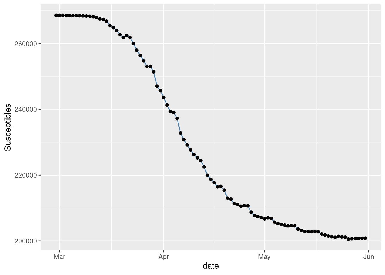
Figure 1: Observed Susceptibles in NYC.
Figure 2 with the observed time series of Infectives.
gplot(SIR,SIR$t,SIR$I,ylab="Infectives")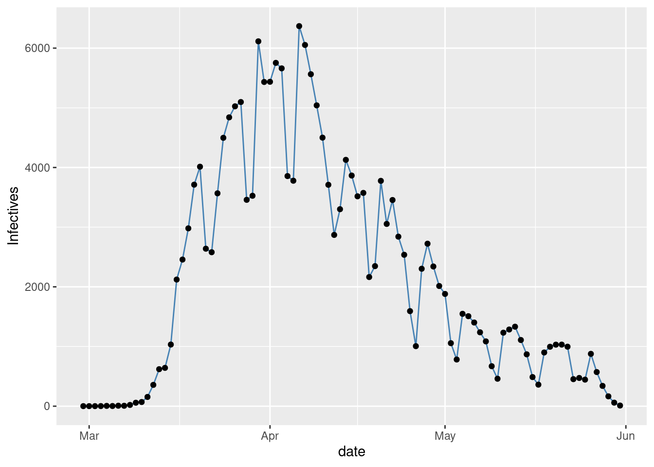
Figure 2: Observed Infectives in NYC.
Figure 3 with the observed time series of Removed.
gplot(SIR,SIR$t,SIR$R,ylab="Removed")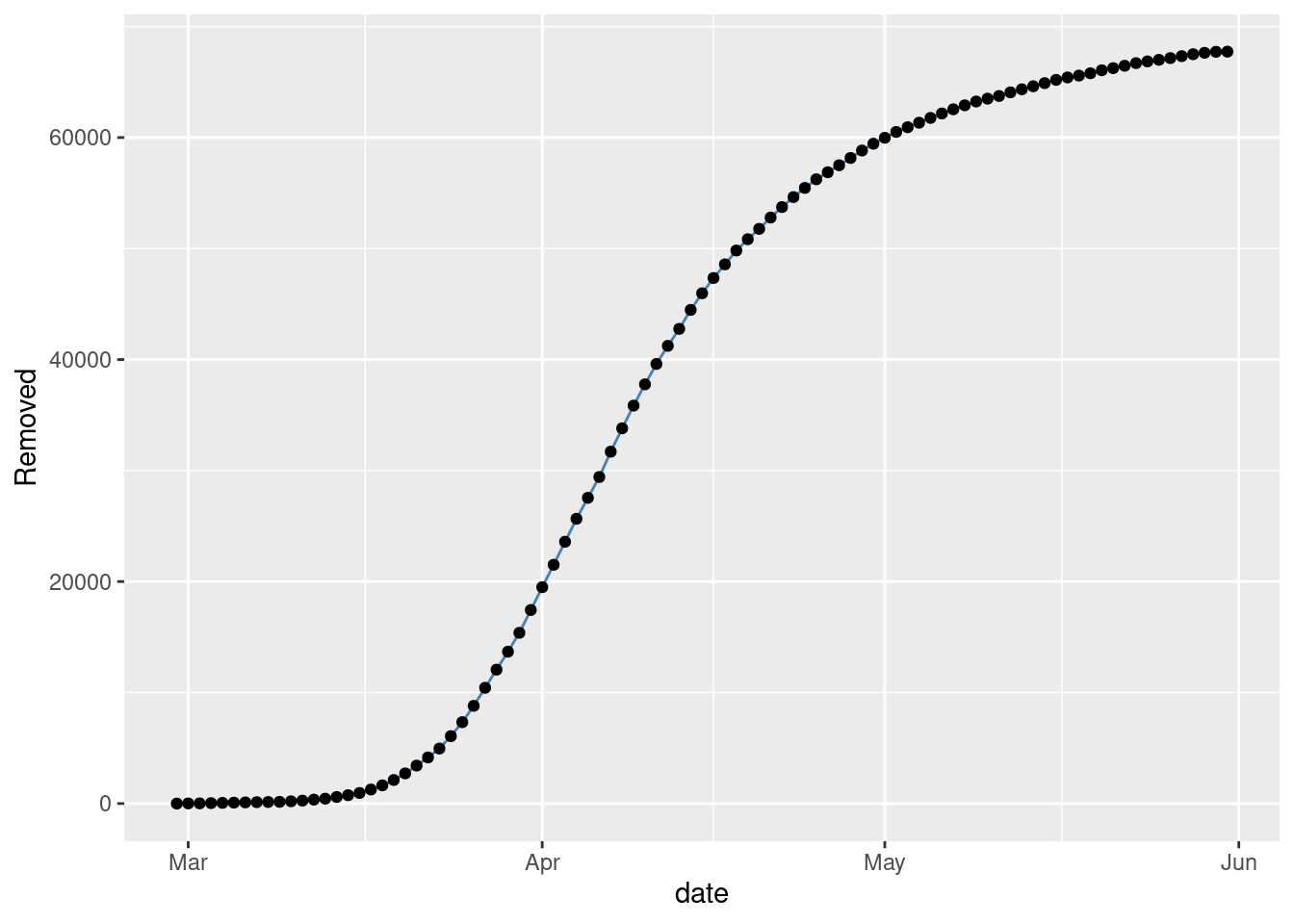
Figure 3: Observed Removed in NYC.
These plots follow the expected shapes for the SIR model. The smoothness of \(R\) and also of \(S\) to a lesser extend, is due to our drastic assumption that \(N\) is the total number of observed individuals.
The noise in the observations is clearly displayed by Figure 2 of the number of Infectives. A gamma plus noise model looks like a good fit. The noise seems to be non stationary however, low at the begining then large and finally a bit smaller at the end. An alternative could be to fit a gaussian process with a prior adapting to the observed noise. Will look at that later. Now just take a look at the raw observed time series of \(R_{0}\)’s, varying with \(t\).
The observed time series of \(R_{0}(t)\)
\(R_{0}(t)\) is shown in Figure 4.
gplot(SIR,SIR$t,SIR$R0,ylab="R_0") +
  geom_hline(yintercept=1, col="red")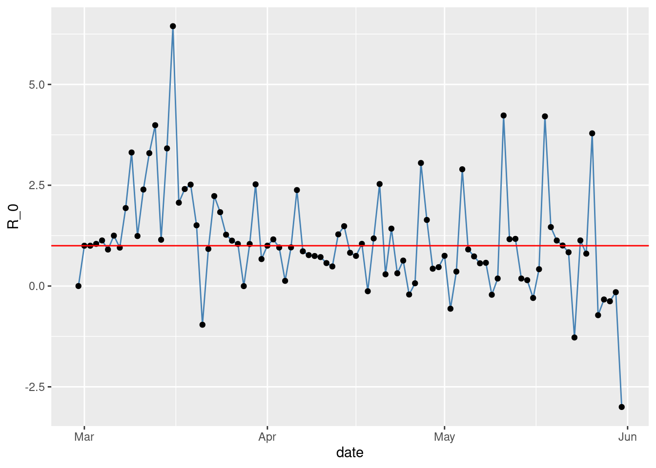
Figure 4: Observed \(R_{0}\) in NYC.
Gaussian Process smoothing of \(R_{0}\)
We start with a brute force fixing of the prior parameters to get a (over) heavy smoothing of the observed raw \(R_{0}(t)\).
functions {
  vector gp_pred_rng(real[] x2,
                     vector y1, real[] x1,
                     real alpha, real rho, real sigma, real delta) {
    int N1 = rows(y1);
    int N2 = size(x2);
    vector[N2] f2;
    {
      matrix[N1, N1] K =   cov_exp_quad(x1, alpha, rho)
                         + diag_matrix(rep_vector(square(sigma), N1));
      matrix[N1, N1] L_K = cholesky_decompose(K);

      vector[N1] L_K_div_y1 = mdivide_left_tri_low(L_K, y1);
      vector[N1] K_div_y1 = mdivide_right_tri_low(L_K_div_y1', L_K)';
      matrix[N1, N2] k_x1_x2 = cov_exp_quad(x1, x2, alpha, rho);
      vector[N2] f2_mu = (k_x1_x2' * K_div_y1);
      matrix[N1, N2] v_pred = mdivide_left_tri_low(L_K, k_x1_x2);
      matrix[N2, N2] cov_f2 =   cov_exp_quad(x2, alpha, rho) - v_pred' * v_pred
                              + diag_matrix(rep_vector(delta, N2));
      f2 = multi_normal_rng(f2_mu, cov_f2);
    }
    return f2;
  }
}

data {
  int<lower=1> N;
  real x[N];
  vector[N] y;

  int<lower=1> N_predict;
  real x_predict[N_predict];

  real<lower=0> rho;
  real<lower=0> alpha;
  real<lower=0> sigma;
}

transformed data {
  matrix[N, N] cov =   cov_exp_quad(x, alpha, rho)
                     + diag_matrix(rep_vector(1e-10, N));
  matrix[N, N] L_cov = cholesky_decompose(cov);
}

parameters {}
model {}

generated quantities {
  vector[N_predict] f_predict = gp_pred_rng(x_predict, y, x, alpha, rho, sigma, 1e-10);
  vector[N_predict] y_predict;

  for (n in 1:N_predict)
    y_predict[n] = normal_rng(f_predict[n], sigma);
}
The above provides the stan code for getting the predictions with the fitted gaussian process.
library(rstan)## Loading required package: StanHeaders## rstan (Version 2.19.3, GitRev: 2e1f913d3ca3)## For execution on a local, multicore CPU with excess RAM we recommend calling
## options(mc.cores = parallel::detectCores()).
## To avoid recompilation of unchanged Stan programs, we recommend calling
## rstan_options(auto_write = TRUE)```r options(mc.cores = parallel::detectCores()) #To avoid recompilation of unchanged Stan programs, we recommend calling rstan_options(auto_write = TRUE)
N <- nd # number of days x = 1:N y = SIR$R0 N_predict = 500 x_predict = sort(runif(N_predict,1,N))
pred_data <- list(alpha=1.0, rho=5.0, sigma=2.0, N=N, x=x, y=y,
N_predict=N_predict, x_predict=x_predict)
pred_fit <- sampling(predict_gauss, data=pred_da—
title: covid19
author: Carlos C. Rodriguez
date: ‘2020-05-22’
slug: covid19
categories: [“R”]
tags: [“Rmarkdown”,“blogdown”]
—
We are after the Reproductive number \(R_{0}\) for NYC. We want good reliable estimates given the available data.
First a quick reminder of SIR model.
The SIR epidemic model assumes a fix number \(N\) of individuals are (at each time \(t\)) divided into three groups \((S,I,R)\) thus its name. Where \(S=S(t)\) are the Susceptible individuals that are able to catch the virus, \(I=I(t)\) are the Infectives able to transmit the virus, and \(R=R(t)\) are the Removed individuals that either died or become immune to the virus. It is assumed that \(N=S+I+R\) is constant for all \(t\) and that the changes (\(\delta U = U(t+1)-U(t)\)) satisfy
\[\begin{aligned} \delta S &= -a S\cdot I\\ \delta I &= a S\cdot I - b I\\ \delta R &= b I \end{aligned}\]where \(a,b\) are the parameters of the epidemic. These equations have a simple interpretation. The first one says that \(S\) decreases proportional to the number \(SI\) of matches of \(S\) with \(I\) individuals. The second says that \(I\) increases by the same amount discounting for the \(R\) that are removed at that time given by the third equation. The most important parameter of the epidemic is not \(a\) or \(b\) but their ratio: \(R_{0}= (a/b)S\) known as the reproductive number or \(R_{0}\) (read R-naught) made famous by the movie Contagion. The infection is exploding or dying out depending on \(R_{0}>1\) or \(R_{0}<1\) since the second equation says that \(I\) is increasing (\(\delta I >0\)) or decreasing (\(\delta I < 0\)) depending on \(R_{0}\).
Learn more about SIR. HINT Use the internet.
Get some data
library(ggplot2)
nyc_url <- "https://github.com/nychealth/coronavirus-data/"
nyc_url_raw <- paste(nyc_url,"raw/master/",sep='')
nyc_csv <- "case-hosp-death.csv"
nycdata <- paste(nyc_url_raw,nyc_csv,sep='')

# nycdata <-
#   "https://github.com/nychealth/coronavirus-data/
#          raw/master/
#          case-hosp-death.csv"

hosp <- read.csv(nycdata,header=T)

# USAGE: gplot(SIR,SIR$t,SIR$S,ylab="Susceptibles")
gplot <- function(df,t,y,xlab="date",ylab="y") {
    p <- ggplot(df, aes(x=as.Date(t,"%m/%d/%y"), y=y)) +
        geom_line( color="steelblue") +
        geom_point() +
        xlab(xlab) +
        ylab(ylab)
    p
}

# approx SIR.

hosp[is.na(hosp)] <- 0
nc = hosp$C         # new cases
nh = hosp$H        # new hospitalizations
nd = hosp$DE      # new deaths

N = sum(nc+nh+nd)       # total
R = cumsum(nh+nd)-nh            # Removed
I = nc                                   # Infectives
I[which(I==0)] <- 1     # regularize to 1.
S = N - R - I                       # Susceptible

SIR <- data.frame(t=hosp$DATE,S=S,I=I,R=R)
# add t=0
R = c(0,R)
S = c(N-1,S)
I = c(1,I)
ndays1 <- length(I)
nd <- ndays1-1

a = -diff(S)/(S*I)[1:nd]
b = -(diff(S)+diff(I))/I[1:nd]
b[1] <- 1   # otherwise division by 0 below...
R0 = (a/b)*S[1:nd]
SIR$R0 <- R0
Approximate SIR from the available data
The reported numbers of daily cases, hospitalizations, and deaths are clearly under representing the actual numbers for New York City. We ignore this as a first approximation.
The total number \(N\) for the population of NYC is also uncertain and obviously not constant. We make the drastic assumption that the total number of observations is \(N\). We start from here but will look at more realistic models later.
\(S,I,R\) plots:
See Figure 1 showing the observed timeR0 = (a/b)*S[1:nd]
series of Susceptibles.
gplot(SIR,SIR$t,SIR$S,ylab="Susceptibles")Figure 1: Observed Susceptibles in NYC.
Figure 2 with the observed time series of Infectives.
gplot(SIR,SIR$t,SIR$I,ylab="Infectives")Figure 2: Observed Infectives in NYC.
Figure 3 with the observed time series of Removed.
gplot(SIR,SIR$t,SIR$R,ylab="Removed")Figure 3: Observed Removed in NYC.
These plots follow the expected shapes for the SIR model. The smoothness of \(R\) and also of \(S\) to a lesser extend, is due to our drastic assumption that \(N\) is the total number of observed individuals.
The noise in the observations is clearly displayed by Figure 2 of the number of Infectives. A gamma plus noise model looks like a good fit. The noise seems to be non stationary however, low at the begining then large and finally a bit smaller at the end. An alternative could be to fit a gaussian process with a prior adapting to the observed noise. Will look at that later. Now just take a look at the raw observed time series of \(R_{0}\)’s, varying with \(t\).
The observed time series of \(R_{0}(t)\)
\(R_{0}(t)\) is shown in Figure 4.
gplot(SIR,SIR$t,SIR$R0,ylab="R_0") +
  geom_hline(yintercept=1, col="red")
Figure 4: Observed \(R_{0}\) in NYC.
Gaussian Process smoothing of \(R_{0}\)
We start with a brute force fixing of the prior parameters to get a (over) heavy smoothing of the observed raw \(R_{0}(t)\).
functions {
  vector gp_pred_rng(real[] x2,
                     vector y1, real[] x1,
                     real alpha, real rho, real sigma, real delta) {
    int N1 = rows(y1);
    int N2 = size(x2);
    vector[N2] f2;
    {
      matrix[N1, N1] K =   cov_exp_quad(x1, alpha, rho)
                         + diag_matrix(rep_vector(square(sigma), N1));
      matrix[N1, N1] L_K = cholesky_decompose(K);

      vector[N1] L_K_div_y1 = mdivide_left_tri_low(L_K, y1);
      vector[N1] K_div_y1 = mdivide_right_tri_low(L_K_div_y1', L_K)';
      matrix[N1, N2] k_x1_x2 = cov_exp_quad(x1, x2, alpha, rho);
      vector[N2] f2_mu = (k_x1_x2' * K_div_y1);
      matrix[N1, N2] v_pred = mdivide_left_tri_low(L_K, k_x1_x2);
      matrix[N2, N2] cov_f2 =   cov_exp_quad(x2, alpha, rho) - v_pred' * v_pred
                              + diag_matrix(rep_vector(delta, N2));
      f2 = multi_normal_rng(f2_mu, cov_f2);
    }
    return f2;
  }
}

data {
  int<lower=1> N;
  real x[N];
  vector[N] y;

  int<lower=1> N_predict;
  real x_predict[N_predict];

  real<lower=0> rho;
  real<lower=0> alpha;
  real<lower=0> sigma;
}

transformed data {
  matrix[N, N] cov =   cov_exp_quad(x, alpha, rho)
                     + diag_matrix(rep_vector(1e-10, N));
  matrix[N, N] L_cov = cholesky_decompose(cov);
}

parameters {}
model {}

generated quantities {
  vector[N_predict] f_predict = gp_pred_rng(x_predict, y, x, alpha, rho, sigma, 1e-10);
  vector[N_predict] y_predict;

  for (n in 1:N_predict)
    y_predict[n] = normal_rng(f_predict[n], sigma);
}
The above provides the stan code for getting the predictions with the fitted gaussian process.
library(rstan)## Loading required package: StanHeaders## rstan (Version 2.19.3, GitRev: 2e1f913d3ca3)## For execution on a local, multicore CPU with excess RAM we recommend calling
## options(mc.cores = parallel::detectCores()).
## To avoid recompilation of unchanged Stan programs, we recommend calling
## rstan_options(auto_write = TRUE)options(mc.cores = parallel::detectCores())
#To avoid recompilation of unchanged Stan programs, we recommend calling
rstan_options(auto_write = TRUE)
N <- nd # number of days
x = 1:N
y = SIR$R0
N_predict = 500
x_predict = sort(runif(N_predict,1,N))
pred_data <- list(alpha=1.0, rho=5.0, sigma=2.0, N=N, x=x, y=y,
N_predict=N_predict, x_predict=x_predict)
pred_fit <- sampling(predict_gauss, data=pred_data, iter=1000, warmup=0,
chains=1, seed=5838298, refresh=1000, algorithm="Fixed_param")##
## SAMPLING FOR MODEL 'b42a8c10415d8faa784e9ab59a64657f' NOW (CHAIN 1).
## Chain 1: Iteration: 1 / 1000 [ 0%] (Sampling)
## Chain 1: Iteration: 1000 / 1000 [100%] (Sampling)
## Chain 1:
## Chain 1: Elapsed Time: 0 seconds (Warm-up)
## Chain 1: 13.346 seconds (Sampling)
## Chain 1: 13.346 seconds (Total)
## Chain 1:#source("gp_util.R")
# Plot Gaussian process realizations
plotgpfit <- function(fit,x_predict,title,...) {
params <- extract(fit)
I <- length(params$f_predict[,1])
c_superfine <- c("#8F272705")
plot(1, type="n", main=title,
xlim=c(1, N), ylim=c(-2, 6.8),...)
for (i in 1:I)
lines(x_predict, params$f_predict[i,], col=c_superfine)
abline(h=1)
meanf <- colMeans(params$f_predict)
lines(x_predict,meanf)
}Figure 5
plotgpfit(pred_fit,x_predict,"Posterior: R0 NYC",
ylab="R_0", xlab="days after 02/29/2020")
points(x=1:N,y=SIR$R0)
Figure 5: Posterior R0
Let’s get some useful statistics from the predictions,
meanf <- colMeans(extract(pred_fit)$f_predict)
tpeak=round(x_predict[which(meanf==max(meanf))])
SIR$t[tpeak] # 3/14/20## [1] 03/14/2020
## 91 Levels: 02/29/2020 03/01/2020 03/02/2020 03/03/2020 ... 05/29/2020Summary:
The posterior mean of \(R_{0}\) shows that it took about two weeks from the first detected case for the epidemic to reach the peak on March 14.
It took another two weeks to get back to \(R_{0}=1\) and the NY state Executive Order to stay at home was only set on March 22, days after the epidemic started dying out. These are very rough estimates as good only as the assumptions on which the model is based. But they seem to say that the goverment intervention has not been able to make a difference. It seems that the epidemic in NYC is running its course regardless of the 6 feet of separation.
Aknowledgement:
The GP stan code is lifted from, Michael Betancourt ) ta, iter=1000, warmup=0, chains=1, seed=5838298, refresh=1000, algorithm=“Fixed_param”)
SAMPLING FOR MODEL ‘b42a8c10415d8faa784e9ab59a64657f’ NOW (CHAIN 1).
Chain 1: Iteration: 1 / 1000 [ 0%] (Sampling)
Chain 1: Iteration: 1000 / 1000 [100%] (Sampling)
Chain 1:
Chain 1: Elapsed Time: 0 seconds (Warm-up)
Chain 1: 13.346 seconds (Sampling)
Chain 1: 13.346 seconds (Total)
Chain 1:
```
#source("gp_util.R")
# Plot Gaussian process realizations
plotgpfit <- function(fit,x_predict,title,...) {
    params <- extract(fit)
    I <- length(params$f_predict[,1])

  c_superfine <- c("#8F272705")
  plot(1, type="n", main=title,
       xlim=c(1, N), ylim=c(-2, 6.8),...)
  for (i in 1:I)
      lines(x_predict, params$f_predict[i,], col=c_superfine)

  abline(h=1)
  meanf <- colMeans(params$f_predict)
  lines(x_predict,meanf)
}
Figure 5
plotgpfit(pred_fit,x_predict,"Posterior: R0 NYC",
          ylab="R_0", xlab="days after 02/29/2020")
points(x=1:N,y=SIR$R0)
Figure 5: Posterior R0
Let’s get some useful statistics from the predictions,
meanf <- colMeans(extract(pred_fit)$f_predict)
tpeak=round(x_predict[which(meanf==max(meanf))])
SIR$t[tpeak]   # 3/14/20
## [1] 03/14/2020
## 91 Levels: 02/29/2020 03/01/2020 03/02/2020 03/03/2020 ... 05/29/2020Summary:
The posterior mean of \(R_{0}\) shows that it took about two weeks from the first detected case for the epidemic to reach the peak on March 14.
It took another two weeks to get back to \(R_{0}=1\) and the NY state Executive Order to stay at home was only set on March 22, days after the epidemic started dying out. These are very rough estimates as good only as the assumptions on which the model is based. But they seem to say that the goverment intervention has not been able to make a difference. It seems that the epidemic in NYC is running its course regardless of the 6 feet of separation.
Aknowledgement:
The GP stan code is lifted from, Michael Betancourt )